How do we change the raw measurements into relative humidity?

First, we have to admit that you will be missing one measurement that you will have to estimate, perhaps by referring to local weather information. That is barometric pressure. A good electronic barometer is rather expensive and we don't have one.

We take the following derivation of relative humidity directly from ASAE STANDARDS 1985, 32nd Edition, American Society of Agricultural Engineers, St. Joseph, MI, pp 34-35.

Intimidating, isn't it? There are several ways to do this. One can program it on a computer in BASIC, FORTRAN or C. One can calculate it in a spreadsheet. One cannot use instruction 12 on the CR10X datalogger in this lab, because it applies only to a special temperature and relative humidity sensor made by Campbell Scientific. Setting this up in a spreadsheet is best, and good practice for you. Break it down equation by equation, step by step from [25] back up to [20]. You should have a spreadsheet with three input cells, Patm, Tw and Td. It should calculate the intermediate values of hv, b, Pv and Ps, and then the final value of rh. Notice that the range of our interest is 273.15 °K to 323.15 °K, which means that you do not have to use the equations of other ranges. You should set them up in one column apiece so that you can handle more than one set of values.

Now, you have to take some data, using the thermistor bridge circuits you have already designed, built and calibrated. Four thermistor assemblies, like that shown in Figure 10, were constructed for this lab, labeled A, B, C and D. You will have used one of them in your calibration exercise, and should have kept the bridge circuit you designed undisturbed for this lab. You must use the same thermistor assembly and bridge circuit. For this exercise, you will assemble it with a plastic PVC venturi assembly that includes a cotton wick for the wet bulb measurement. You will use two different fans and no fan to investigate the effect of aspiration on the measurement. You will use a mercury barometer to get basic atmospheric pressure, and use a manometer to investigate the change in air pressure in the venturi. If one can be found, you will compare the results to a sling psychrometer.

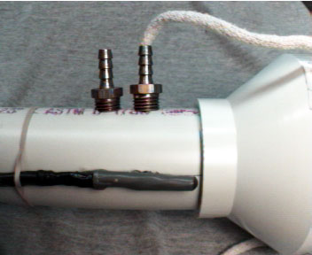
In general, we must have some air movement to cause evaporation from the wet bulb and produce the wet bulb temperature depression. We will accomplish this with a fan pulling air through a venturi tube in which the thermistors are placed. Figure 17 shows such a venturi tube, made from common PVC plumbing pipe and fittings, with a thermistor assembly attached at the top. As air is drawn from the left through a 3-inch to 1-1/2-inch reducer, it will speed up due to same mass moving through a smaller opening.

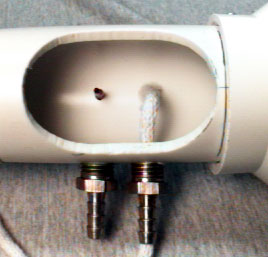
The thermistors on the assembly pass through two holes in the side of the 1-1/2-inch tube, as shown in Figure 18. Here, the thermistors are the two black dots seen through an oval access door cut in the side of the tube. Below them, two 1/4-inch brass hose connectors are threaded into the tube. As the air passes from left to right, it must pass over the dry thermistor first. The venturi effect causes a drop in air pressure in the tube as the air speeds up, that will increase the drop caused by the suction of the fan. The first hose connector under the dry thermistor will be connected to a manometer to measure the drop.

 

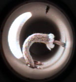
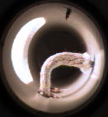
A cotton wick made from clothesline rope passes through the second hose connector. The wick is a hollow braid from which the synthetic core has been removed. Figure 19 shows the braid being pushed over the wet bulb. You will have a container of deionized water into which you will drop the braid. You must use deionized water to avoid any reduction in the efficiency of the wick due to salt crystallization. The water will wick up the braid. As air passes over the braid in the venturi tube, the water will evaporate and cool the wet thermistor. Normally, one saves water and power by starting the fan just before the measurement. You will measure how long it takes for the measurement to settle for different size fans and no fan.

 

Figure 20 shows a piece of sheet aluminum onto which the oval cutout from the venturi tube access door has been screwed. It serves three purposes. It holds the door in place and covers the access hole. It helps to hold the thermistor assembly in place. When the green ground wire is connected to it, it also provides an electrostatic shield for the thermistor assembly that cuts down on any noise pickup. Figure 21 shows the installation steps. First pull the wick through the taped hole, and pull the taped hole down over the hose connectors. Be careful; the edges of the metal can cut flesh. Pull the shield over the thermistor assembly and around until the plastic door clicks into place in the hole. Tighten the shield by pulling from the door towards the hose connectors. Secure the shield with tape, rubber band or a stainless steel hose clamp. Connect the green ground wire to the shield by wedging it under the shield or steel hose clamp.

 

Figure 22 shows the two fans you will use. The smaller fan, an NMB model 2410ML-04W-B10-P00, is mounted inside a length of 3-inch schedule 40 PVC pipe. It is rated at 12 VDC, 100 mA, 14 cubic feet per minute. The direction of air flow is from the fan into the pipe. You will insert the that end of the pipe into the 1-1/2-inch to 3-inch adapter on the venturi assembly closest to the thermistors. The larger fan, a Radio Shack No. 273-243B, is rated at 12 VDC, 160 mA, 26 cubic feet per minute. It is mounted on the downstream end of its tube, which should be inserted in the same place on the venturi assembly, with the fan on the other end of its tube.

 

There are three venturi assemblies, labeled 1, 2 and 3. For this exercise, assemble your bridge circuits and connect them to the datalogger as before in Figure 11. Also connect the Start Button to the datalogger as in Figure 15. Instead of the doohickey in Figure 16, connect the fans between the switched 12V and ground terminals on the datalogger, the red wires to SW +12 V and the black wires to G. Set up your assemblies on lab stands in such a way that none will suck in the exhaust of any other. Set up a beaker or test tube of deionized water as close below the venturi tube as possible and put the cotton wick in it. Set up a water manometer and attach it to the hose connection under the dry thermistor. You will each take turns taking data with no fan, the small fan and the large fan. This will give you all data for three levels of aspiration for each thermistor assembly.

Now download the datalogger program thrmfan.dld (Listing 3) from the computer to the datalogger, using the pc208e software. This time when you push the Start Button, the program will turn on the fans instead of the doohickey and take data only for as long as you hold the button down. It will take data continuously, saving the variables, stmin, stsec, Vra, Vrb, ..., Vrf, corresponding to the minute and second when the datalogger begins to measure the bridge voltage ratios, Vra, ..., Vrf.

Using the pc208e software, go into monitor mode and observe locations 1-8, corresponding to stmin, stsec, the start time in minute of the day and second of the minute, and Vra through Vrf, the voltage ratios taken with the three-wire bridge instruction, P5. The program will only store data when the Start Button is pushed, but will generate data continuously to monitor. You should see the wet thermistor readings, in particular, for those assemblies with fans, change as the evaporation cools the thermistor. When you release the button, notice whether or not the wet thermistor reading returns to the still air value faster or slower than it dropped with the fan on. Because it must take heat from still air to come back up to room temperature, the change should be slower after the fan is turned off.

This is important. Changes like this typically go as shown in equation [28]. Say the thermistors have settled to room temperature plus that due to internal heating with the fan off. When the fan is turned on, evaporation begins to cool the wick and wet thermistor and its temperature drops. Eventually, it equilibrates to the steady-state conditions set by the air temperature, humidity and flow. If it does so according to [28] then it reaches 98% of the final change in values at about t = 4*tc.

If you are making a measurement in the field, where power for the fan is at a premium, then you want the fan on just long enough for the measurement to settle, about four or five times the practical time constant. Or maybe twice that. Because, if the fan is not on long enough, the measurement will not have settled and will not be accurate. There may, for example, be a heat buildup from solar heating in the psychrometer box, which needs to be flushed out with the fan to make an accurate measurement. Further, when you are making this measurement in the lab, and are trying to figure out the time constant, you need to leave the fan off long enough between measurements for the wet thermistor to warm back up to room temperature. Otherwise, you will not have enough difference between Vi and Vf for the wet bulb voltage ratio to be able to tell when it settles after the fan is turned on.

You may find the there is enough temperature variation in the lab air, possibly from a number of warm bodies in the area, that it is not clear when the wet and dry thermistors have settled to their final values. In that case, you will have to take data long enough to be sure. The dry thermistor will settle much faster than the wet thermistor because it has a much smaller thermal mass than the wet thermistor plus the wet wick. So, the practical measurement of time constant for the psychrometer is the difference between the wet and dry thermistors, or the wet bulb depression. In variable air, both thermistors will change, but the difference between them will likely change only until the wet thermistor has equilibrated with the relative humidity.

Consider also that field conditions will require you to use some kind of filter to keep both dust and insects out of the works. We will simulate that by covering the intake end of the venturi assembly with a coffee filter, held in place by a rubber band. We will also simulate clogging of the filter by dust and other debris with a cardboard restriction. You will do the runs for no filter, a single coffee filter, and a coffee filter over a cardboard restriction representing a 90% clogging of the filter. Consider that restriction of the airflow will likely increase the time constants, and take data accordingly.

Realize that three conditions of fan size or presence and three conditions of intake flow restriction will mean nine runs per setup. Since the runs can be done simultaneously on all three setups, cooperation in and among the groups is essential. Each group should make up a 3x3 matrix and check off each combination as it is run. You should start with the 90% clogged coffee filter, changing out the fans, so that the time constants will be getting smaller with remaining runs.

Do a few practice runs to get an idea of how the time constants will change with fan presence or size. You may be able to reduce the time between runs by breathing into the psychrometer. Don't spit on the dry thermistor. The idea is to see a large enough change when the fans come on to determine time constants. You will also be doing more than just changing fans around, so work out an efficient approach. Practice uploading data from the datalogger to the computer after each run to the cr10lab.dat file, then renaming it to a something distinctive to the run.

You will be using your time series data to determine the psychrometer time constant, tc, by fitting the measured data to equation [28]. If you have no other curve-fitting software, you can use the Quattro Pro 2.0 for DOS spreadsheet, crvfit.wq1. It shows a fit of y^ (Vr in [28]) to y(t) using the same /data/solve facility you used in the bridge design spreadsheets. Notice that the time series data is t in A9..A89 and y(t) in B9..B89. The estimated initial value of y, yi, the final settled value of y, yf, and the time constant, tc, are in cells C4, C5 and C6, respectively. These are used to calculate the estimated y(t), y^, in C9..C89. The difference, del-y = y^-y(t), is calculated in D9..D89, with the sum of squares of del-y in cell D6. This cell, D6, is the formula cell for /data/solve. Cells C4..C6 are the variable cells.

You will have to use some common sense in using this spreadsheet. As with the bridge design spreadsheets, you have to start with an estimate of (yi, yf, tc) reasonably close to the best answer to get to the best answer. In this spreadsheet, the y(t) data came from (yi, yf, tc) = (0,1,1) with a random number noise added. You can see that the solve-for method has settled on bogus values, because the starting values were too far off. You will have to plot the data and the fit against time and manually adjust the three curve fit parameters to a reasonable fit before applying the spreadsheet solve-for method. You can expect this to be more difficult if you have a noisy measurement, or if you did not take enough data to get reasonably close to a settled value, yf.

Exercise 2

1. Assemble the psychrometer from the thermistor and venturi tube assemblies, connect the thermistors, Start Button and fans to the datalogger, and load the program thrmfan.dld into the datalogger. Connect the manometers to the venturi tubes and place the wicks in deionized water.
2. Cover the intake of each psychrometer with a circle of manila folder cardboard, 4 in diameter, from which a circle of 0.58 in radius has been cut from the center. Verify by measuring the intake that this represents a reduction of the intake area to about 10%. Cover the intake and the cardboard restriction with a coffee filter. Hold the coffee filter in place with a rubber band.
3. Attach the two fans to one setup and leave the third without.
4. Practice taking and uploading data, until you have an idea of how long the run should be to assure that the psychrometer time constant can be determined by fitting the wet thermistor depression to equation [28]. Realize that the setup without a fan will have an irrelevant and likely infinite time constant. So take data for it but do not use it to determine the length of the run.
5. Make sure that all the data from the datalogger is uploaded and renamed in a separate file before doing each measurement run.
6. Take the barometric pressure at the beginning of the measurement runs, and the end, and at each hour in between.
7. Take manometer readings from the each psychrometer while the fans are on during each run.
8. Take sling psychrometer readings during each run. Use deionized water on the wet bulb.
9. Make sure the datalogger date and time correspond to real time and write down the time with the beginning of each run, associated with the data filename. If you don't know how to do this, look at the practice data file variables stmin (minute of the day) and stsec. Count the time between runs.
10. With the coffee filter and 90% restriction in place, do one run each with no fan, the small fan and the large fan on each setup.
11. With the coffee filter alone in place, do one run each with no fan, the small fan and the large fan on each setup.
12. With no filter in place, repeat 9.
13. Now, just for fun, use the two 4-inch lengths of 3-inch schedule 40 PVC pipe to connect all the psychrometers together in series. Use just one coffee filter on the intake and the large fan on the outlet. As the air passes over each wick, it should become cooler and more humid. Does it? By how much? Run this experiment three times, rotating the psychrometers in order so that each setup gets a run from each position. Be sure to take manometer data and barometric pressure.
14. Process your data. Use the calibration equations you developed and equations [20]-[27] to calculate dry bulb temperature, wet bulb temperature, wet bulb depression and relative humidity. Use the manometer readings to correct the barometric pressure to the inside of the venturi tubes. Plot these variables and the voltage ratio measurements versus time for each run.
15. Fit your data. Fit the time series for wet bulb depression to equation [28] for each run. Determine the time constant, tc, for each psychrometer for each combination of fan and filter restriction. Comment on the effects. Comment on how long the each fan should run before taking wet and dry thermistor readings to assure an accurate estimate of relative humidity under a variety of conditions. Realize that you have taken data for a limited set of conditions, not representative of the full range of possible field measurements.
16. Compare your data to the sling psychrometer. Use the settled values of temperature and relative humidity at the end of each run, just before the fan is turned off. Show tables of wet and dry bulb errors, and relative humidity errors for each fan and filter combination, taking the sling psychrometer and barometric pressure readings as correct. Comment on the possible sources of the errors.
17. Plot and analyze the data from runs with the psychrometers in series. You may exchange data between groups, or use just your own data from each position. Was there any significant increase in humidity or decrease in air temperature from the intake to the exhaust? Was there any discernable change in time constant from position to position? If so, what implication might this have for field measurements?
18. Also take the runs with the large fan and show whether or not the drop in air pressure inside the venturi tube had any significant effect on the measurement of relative humidity. If so, would you recommend that the pressure be measured inside the venturi tube to compensate?
19. Make recommendations for simple and effective methods by which a wider range of temperature and humidity conditions could be measured and investigated in the laboratory.
20. Make recommendations for improving this exercise for future students.