5. Take the ice point measurements from the thermistors and adjust the bridge circuits to +Vspan.

The ice bath should be starting to melt by this time. Make sure that the thermistors have ice around them. If they are in water below the ice, either pull them up, or dump some water and add some ice. If the ice is frozen about them, gently break it up or thaw it before moving them. It may help to have some circulation of water about the thermistors, provided by perhaps a magnetic stirring bar in water below the ice, going at slow speed.

The entire lab may have to watch the same screen of the pc208e software in monitor mode. Let's assume that your intended Vspan is ± 250 mV, and the excitation, Vs, is 2000 mV. Let's also assume that your design puts 0 °C at +250 mV. If you are adjusting the bridge designated "a" in Figure 11, then Rta should be +250/2000 = +0.125000 when the thermistor is at 0 °C. You can adjust your bridge several ways. You can add fixed resistors either in series or parallel to get R1 or R2, or you can add a pot in series or parallel, and adjust it with a small screwdriver (bring one to lab). Get familiar before the lab with equations [9] and [10]. Then adjust your bridge circuits by trial and error to achieve the proper voltage ratio, Rt*. Try to get it within three significant digits, preferably four. Then let the calibration to the SPRT take up the slack.

6. Connect the SPRT to the datalogger and download the temperature calibration program.

Figure 14 shows the connection of the SPRT and its bridge circuit to the CR10X. The terminals are labeled left to right as they are on the CR10X. The color labels next to the terminals are wire colors. The R and B farther down indicate either RED or BLACK colored tape on the jackets of the two cables used. The green wires going to the ground terminals, G, are connected to the cable shields.

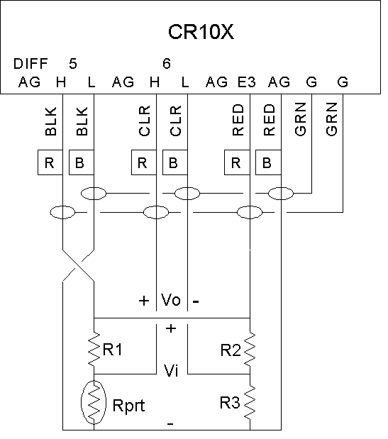
This circuit generates a drive voltage of 2000 mV between the excitation, E1, and analog ground, AG, terminals. To cancel out any voltage drop in the cables themselves, the input voltage to the bridge, Vi, is measured on differential input channel 5. The bridge output voltage is measured on a ±  2.5 mV range, with 60 Hz rejection, on differential input channel 6. Instruction P09 does the measurement and produces 1000*Vo/Vi.

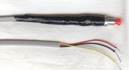
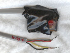
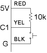
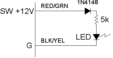
In addition you will add two moredevices, a start button (Figure 15a,b) and a doohickey (Figure 16a,b). Connect the black, red and yellow wires of the start button to the G, 5V and C1 terminals, respectively, on the block on the lower right-hand corner of the datalogger. Use a wire to make a connection between the C8 and "SWITCHED 12V CONTROL" terminals on the same block. On the upper right-hand terminal block, connect the red/green lead of the doohickey to "SWITCHED 12V", and the black/yellow lead to G. When the temperature bath reaches the temperature for a calibration point, pressing the start button will tell the datalogger program to start taking data. The doohickey will light up red and remain lit until the datalogger has finished taking data.

Figure 15a: Start Button	Figure 16b: Doohickey

 

Figure 15b: Start Button Circuit Figure	16b: Doohickey Circuit

Now download the thrmcal.dld program (Listing 2) the same way you did the thrmice.dld program, using the pc208e software. If you follow the program, you can see that once very second, the datalogger takes a temperature reading from the SPRT. It then checks to see if the Start Button is closed. If not, it waits for the next second to do the same thing again. If the button is pressed, it sets C8 high, which causes the Doohickey to light. It then starts a loop of 22. In each loop, it takes measurements of the SPRT and three thermistor pairs in order, ViVo, Vra, Vrb, ..., Vrf. It performs a running average of 20 values with those measurements and places the running average in ViVobar, Vrabar, ..., Vrfbar. Since the loop goes two loops longer than the running average, only the measurements for that press of the button will be used in the average. In the last operation of the loop, the program calculates the SPRT temperature and puts it in Tprt. The start and end times in minutes and seconds are also taken before and after the loop. At the end of the program, the varialbles, Tprt, ViVobar, Vrabar, ..., Vrfbar, are written to output storage, so that you can upload them to a disk file.

7. Move the thermistors to the variable bath and take at least ten different temperature points between 0 and 50 °C.

It takes a long time for the temperature bath you will use to get to lower temperatures. Before you start, it should already be at or below 0 °C. If all goes will, it will be an 8-liter bath with a single dial temperature control, and switches for the heating and cooling parts. When switched on, the cooler runs continuously. It is not necessary much above room temperature. When switched on, the heater runs intermittently, attempting to drive the temperature of the bath to the setting on the dial. With luck it should take about 5 to 10 minutes to raise to each new temperature point.

Using the pc208e software, download the program thrmcal.dld to the datalogger, as you did thermice.dld. Then change the pc208e to monitor mode and monitor locations 1 to 10, variables Tprt, ViVobar, Vrabar, Vrbbar, ..., Vrfbar, stmin and stsec. Your bridge circuits should already be attached to the datalogger in the proper manner. Place the thermistor assemblies in the bath and tape the cables to the side of the bath to maintain their positions in it. The bath has a circulation pump. You don't want the stream to beat your thermistors against the bath walls or each other and cause damage. There is a hole near the refrigeration coils for a thermometer, but it should be as close to the thermistors as possible without picking up any of their dissipated heat. It may be reasonable to tape the thermistor assemblies to the SPRT with the thermistors pointing out in a star pattern.

If the value of ViVobar is something like -99999, then the temperature of the bath is too low and the SPRT measurement is out of range. Increase the temperature a degree at a time, waiting several minutes between, until the SPRT reading becomes normal. You should begin the series within 0.5 °C of 0 °C. If not all of the thermistor bridges are in range, and some read ± 99999, then take your low end measurements about 1 °C apart up to 5 °C until all come into range. You will need at least 10 measurements across the range of 0 °C to 50 °C. but preferably 20.

As noted before, you take the measurement by pressing the Start Button. Wait until the bath temperature varies no more than ± 0.1 °C about an average SPRT reading. When in the monitor mode in the pc208e software, you can press D on the computer keyboard to change the number of significant digits displayed. Make sure that as many as possible are displayed. When the red light on the doohickey goes out, write down stmin, stsec, Tprt, ViVobar, and the two Vr measurements for your bridge. This duplicates the data that the datalogger stores, but the file you will get from it has five significant digits per measurement. Although they may be well below the accuracy of the measurement, the monitor readings will have more significant digits. It's also good practice in case the datalogger data is lost for some reason.

As the temperature of the bath rises, gas will come out of solution and bubbles will likely stick to the thermistors and SPRT. It's a good idea to shake them off before a reading since they are partial insulation. This bath will have antifreeze in it; don't lick your fingers and keep them out of your eyes if they get wet. As noted before, you should be taking measurements every 5 °C. You will notice that the bath may overshoot the temperature set on the dial and oscillate a bit. If this happens, it will be because it takes time for the heater to loose its heat to the bath after the control circuits turn it off. If you see this happening, you can anticipate it by turning the heater off before the SPRT shows the desired temperature. Then turn it back on as the temperature settles. This takes practice and will waste more time for the first few tries than it saves.

We will be pretending that the SPRT is an absolute standard. In reality, it's a cheap model, and bridge resistors are carbon film instead of metal film. You must keep the metal box with the SPRT bridge away from any source of heat. Allowing it to heat up will cause the SPRT reading to rise and make your analysis more difficult. If the temperature of the box is consistent, then so too will be the SPRT measurements. Sticking a thermometer to the box inside insulation and keeping a record of its readings might be a good idea.

8. Upload the measurement data from the datalogger to the computer; transfer to floppy disk.

Every time you pressed the Start Button for longer than one second when thermcal.dld was running on the datalogger, a line with the following 13 variables was written to the datalogger output storage: ID, Tprt, ViVobar, Vrabar, Vrbbar, Vrcbar, Vrdbar, Vrebar, Vrfbar, stmin, stsec, endmin, endsec. The variable ID is a three-digit integer meant to identify the datalogger; it has no value to this measurement. Tprt and ViVobar are the SPRT temperature and bridge voltage ratio, respectively. Vrabar to Vrfbar are the 20-sample means of the three-wire thermistor bridge circuits. The variables stmin and stsec are the minute of the day and second of the minute when the 20-sample means were started. The variables endmin and endsec are the corresponding end times.

Notice in instructions 17, 18 and 19 (P5) in Listing 2 that the thermistor bridge ratios have a multiplier of 100. This is because even the high resolution storage in the datalogger is limited to five significant digits, with one decimal point and no exponents. So if a reading is less than 0.1 in magnitude, the leading zeros take up some of the significant digits. Multiplying the thermistor voltage ratio measurements by 100 assures that the decimal point will end up in the middle of the number. If you like, you can think of Vrabar, ..., Vrfbar, as the voltage ratio percentages.

The internal storage of the datalogger has a 23-bit binary mantissa and 6-bit binary exponent. That gives plenty of mathematical resolution compared to the measurements and storage of constants for calibration. Your primary concern in scaling the numbers you will use is to keep as many significant digits as possible before the final output. This avoids roundoff errors.

You will be using the pc208e software to upload the datalogger readings to the computer. Leave the monitor mode by pressing the ESC key. In pc208e, select DataCollection/CallNow<CurrentStn>. A small window will say "Collecting Data Please Wait", while the lower dark blue window will say how many bytes have been received and how many are left to go. The process is done when the small window disappears and the bytes remaining are zero. Then press ALT-X on the keyboard to exit the pc208e software.

The data will be stored in a file called cr10lab.dat. You should rename it in case you have to do this again. Give it a date name, for example mr1099a1.dat for the first file collected on March 10, 1999. Save it to a floppy disk which you should have brought to the lab. This is the backup for your notebook data, which you should put in a file or spreadsheet of another name.

9. Use JMP or some other curve-fitting program to investigate correcting the thermistor voltage versus temperature curves to the SPRT, using polynomials up to sixth order.

If you are going to use JMP IN to analyze this data, you should add a header line to the data file. If it is the file that you got from the datalogger, the header line should include the 13 labels, ID, Tprt, ViVobar, Vrabar, Vrbbar, Vrcbar, Vrdbar, Vrebar, Vrfbar, stmin, stsec, endmin, endsec. They should be separated by spaces. If you are going to use the file in Quattro Pro, they should also be individually enclosed in quotes: "ID" "Tprt" ... "endsec".

The time variables serve only to distinguish readings and observations, such as the temperature of the SPRT bridge box, that you take in your notes. If you have no exceptional observations, both they and the voltage ratio measurements from experiments not your own can be excluded from the analysis. ViVobar can also be excluded if you determine that it has no effect. Your task will be to use the data to generate a calibration curve that converts from the datalogger reading, in this case voltage ratio, Vr*, back to temperature, in this case Tprt.

If you are using JMP IN, import the data into the spreadsheet. Select Import/Text/Others, then specify "All Files (*.*)" before picking your data file name. Or, enter the data by hand into the spread sheet. Set the modeling type, the box on the top left of the column, to C, continuous. Set the role, the box on the top right of the column of your Vr* variables to X, and Tprt to Y. Choose Analyze/Fit X by Y/. Then choose the fitting type below the graphs successively as Fit Line, Fit Polynomial 2, ..., Fit Polynomial 6. In another table, plot the Root Mean Square Error of the fit against the order of the fit, 1, 2, ..., 6. Discuss why some increases in order work better than others. It will help to click on the right arrow box of the fit and select Plot Residuals. Square the RMS Error to get the Mean Square Error and plot that against order.

10. Calculate the RSS error from all possible sources.

We'll give you a hint. Only the measurement error and the contributions to error in your calibration equation will contribute to the error in calculated temperature. How many are there? What are they? How large are they? How does the calibration equation transform the measurement error to temperature error over the range of 0 °C to 50 °C? You will find it easier to use a spreadsheet for this calculation.

Consider Figure 14, the SPRT bridge circuit. The resistors R1, R2 and R3 have been measured at 7489.8, 7493.8 and 109.5 W, respectively. The input voltage, Vi, is set to 2.000 V. The output voltage, Vo, is in the range of ± 2.5 mV. You know from previous discussion that the digital resolution of a ± measurement is 1 part in 7500 and the analog accuracy is ± 0.1%, or 1 part in 1000. Although it is not, assume for the sake of argument that the transformation from bridge voltage ratio to SPRT temperature is linear. Ignoring all other errors, what does that imply is the accuracy of the SPRT temperature measurement? Use this as the contribution of error from the SPRT reading.

When you have determined the source and size of all the errors, add their magnitudes together as the sum of squares. For example, if you have errors of ± 0.005 °C, ± 0.012 °C and ± 0.060 °C from different sources, their sum-squared error would be ± 0.0614 °C. Use this kind of number to show what order of polynomial you can use and add no more than 10% to the size of the sum-squared error of the temperature measurement.

An additional consideration is measurement scaling. The CR10X datalogger has an instruction that will make a fifth-order polynomial transformation, using coefficients of five significant digits. You can enter six significant digits in a program edited in the pc208e software, but it only shows as five when the datalogger program is displayed with its keypad/display or with the pc208e terminal mode. If you allow the coefficients of the transformation equation to fall outside the range of ± 1.0000 to ± 99999., you will loose significant digits in the coefficients and have a less accurate transformation.

Look at the coefficients that come from your curve-fitting analysis. Do they fall outside that range? If so, you will have to scale the values of Vr* with a constant multiplier so that the result falls in the range of about ± 2. Then you will have to recalculate the polynomial fits to see if that produces the desired range of coefficients. If you read ahead to this point before you did your bridge design, and made sure of this, you may be ahead of the game. You can then apply that multiplier, in parameter 7 of the P5 instruction to measure the 3-wire thermistor bridge, when we use it to measure humidity. If you do not do this, and your coefficients are not all of five significant digits, then you must calculate the resulting addition to the error in the temperature measurement over the 50 °C range, and demonstrate its significance.

For ten points extra credit, use a spreadsheet or JMP IN to determine which terms of the polynomial are most necessary. For example, can you drop the (Vr*)² term without significant increase in error? This can be done by stepwise multiple regression and is just possible with JMP IN or Quattro Pro.