Index

• UNDER CONSTRUCTION - means that the page has been started and has substantive information on it, but has not been finished.
• Previous work done for USDA-ARS
• Weir data files used
• Program and data files- Page with a table of most of the program and data files used in this study in 2007. UNDER CONSTRUCTION
• Short Explanation of Simulated Annealing
• The 6% Fit - A fit of an equation to the entire set of weir data, using novel logistic weighting between channel and jet flow. Mean relative error of 6%.
• Fitted trial head-discharge hydraulic equations - Page with most of the trial head-discharge equations used in 2007 to fit the weir data listed above. UNDER CONSTRUCTION
• Summaries UNDER CONSTRUCTION
• More detailed lab notes on equation fitting UNDER CONSTRUCTION
• Application of 6% Fit to Breached Reservoir Model - Page with 6% fit mathematically applied to 44 by 44 by 2 ft model reservoir with breached dam having 1:1 and 6:1 upstream slopes. Equal initial reservoir volumes. Outflow calculated by 6% fit to reservoir head. Head and volume changes simulated by first-order difference equations. Demonstrates that flow through 6:1 upstream slope with headcut is significantly larger than that through 1:1 upstream slope because of larger effective outflow hole in dam. My former employer said it couldn't be done, and that I had no right to disagree, but more water does flow through a larger hole in the ground.
• Application of Blender Fluid Simulation Package to Breached Reservoir Model - The open-source Blender graphics program for animation has a fluid simulation package to model water-like fluids, based upon the Lattice Boltzmann Method for modeling free surface fluids. It includes the effects of mass, inertia, gravity, waves, viscosity, and surface flow resistance, and thus can form jets at flow constrictions. Although only loosely accurate in physics, it confirms that fact that more water flows through larger holes, as demonstrated by the 6% fit.

Weir data files used:

myallraw.prn - all 2682 measurements, 161 KB

my16rawb.prn - all data with 16 inch breach base widths, 143 KB

raw16hh1.prn - 16 inch data with headcut of 1 foot, most like to have aerated jet, 42 KB

weirdat0.prn - all data with 8 inch and 32 inch breach base widths, 18 KB

weirdat1.prn - weirdat0 plus 16 inch base data for small values of upstream dam slope, mu (H:V), and breach side slope, ms (H:V), 36 KB

weirdat2.prn - all 16 inch base width data, 125 KB, comma-delineated ASCII (CDA)

weirdat3.prn - all 2682 measurements, 8, 16 and 32 inch base widths, 147 KB, CDA

weirdat4.prn - all 8 inch data, 21 KB, CDA

weirdat5.prn - all 32 inch data, 3 KB, CDA

weirdat6.prn - 8 and 16 inch data with steep-sided mu and ms, 34 KB

Program and data files - Page with a table of most of the program and data files used in this study in 2007. UNDER CONSTRUCTION

Fitted equations - Page with most of the trial head-discharge equations used in 2007 to fit the weir data listed above. UNDER CONSTRUCTION

Summaries:

May 24 - July 16, 2001, and Oct 23, 2001 - Jan 30, 2002 -- Work done for USDA-ARS

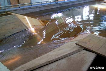
Learn about bernoulli equation and ideal weir equation. Develop equations from integrating the ideal weir equation over the geometric edges of the flume model (June 7, 2001). Fit equations using simulated annealing to sets of weir data taken from 2682 measurements. The weirs were constructed of plywood as prismatic notches in a flume in about 380 different geometries, including base widths of 8, 16 and 32 inches, drops into headcuts of 0, 1/2 and 1 foot, and side and upstream slopes of from 0 up to as much as H:V = 6:1. The experiment took neither velocity data, nor recorded when the "breach jet" was aerated. Aside from physical measurements of the construction of the "dam breach", the experiment measured only the gross flow and upstream height of the water above the breach base, by deliberate choice of the designer. Equations were fitted to data separated into three flow regimes using simulated annealing. Flow with a presumably aerated jet falling into the head cut, by implication because aeration was never recorded. The upstream slope of the "dam" affected this flow, which was the largest for a given upstream water depth. Flow with the breach jet fully in contact with the bottom of the head cut, or notch floor. This flow obeyed that for flow in a trapezoidal channel. And an obvious transition region between the two. In this analysis, upstream bed depth had little apparent effect. This investigator wrote several reports of the findings in research paper format before leaving that employment, most of which are at the "work done" link above.

May 14 - June 11, 2007 -- Redo previous work, developing new equations.

PDF files of the original research notes, dead ends, mistakes and all, are at the "May" and "June" links above. Fit various polynomial equations using simulated annealing to sets of weir data take from the same 2682 measurements. Use objective function, subrouting fcn, based on mean relative error. Investigate weights based on the relative sizes of the upsteam head, he, and the headcut depth, hh, to account for the transition between and effects of fully-aerated jet flow and trapezoidal channel flow. Base equations on dimensionless flow, usually Q/(b*sqrt(g*he^3)). Use a weighting factor of he/(he+hh). Starting May 23, 2007, consider that the relationship is not simple heights, but the relative cross-sectional flow areas of the jet above the breach base, and the headcut (if any) below it. Settle on a weighting ratio, r = (he*he)/(he*he + b*hh), where b is the base width of the breach.

May 28, based on plot of fitted data in Lotus 1-2-3 file, my2807f.123, pick Intermediate Peak and First Order Sequential Formation equations from SPSS TableCurve 2D V4 as possible fitting equations. Go back to polynomial fits occassionally to see relatively unbiased curves and decide upon other functions. Also switch from objective function based on mean relative error to mean absolute error.

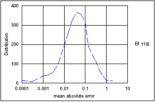
June 4, start plotting log distribution of squared error, and using Chi-Square test to determine best fitting method. Use polynomial fitting functions to look for better method. June 7, choose Logistic Dose Response curve to fit both term with ms only (he^(5/2) term) and term with (ms^2 + mu^2)^(~.4) (approximately he^(3/2), but more like he^4.3).

, with

Q(hat) = calculated breach flow, cfs or ft³/s

b = bottom width of gap in plywood breach, ft

g = acceleration of gravity, 32.174 ft/s²

he = height above the verge of the breach (b) of water upstream, ft

hh = depth of headcut below verge of breach (b), ft

ms = slope of the side of the trapezoidal breach cut, horizontal to vertical, dimensionless

mu = slope of the upstream side of the plywood dam, H:V, dimensionless

D₁ = 0.46342, D₂ = 0.32459, D₃ = -0.16306, D₄ = 0.51441, D₅ = 8.6838,

D₆ = -0.10813, D₇ = 0.73077, D₈ = 0.50789, D₉ = 2.5213, D₁₀ = 0.38428

mean absolute error = 0.08304 CFS

standard deviation of absolute error = 0.13877 CFS

mean relative error = 4.91%, std dev of relative error = 5.94%

Calculated in Fortran simulated annealing program, simanh9.for, with input data file, weirdat3.prn

Plotted results in Lotus 1-2-3 file, jn1107a.123:

Qh = calculated flow, cfs

June 11 to July 1, 2007 -- Developing new equations.

July 1 to 18, 2007 -- Developing new equations.

More Detailed Lab Notes on Equation Fitting - Page with almost daily notes on how the fitting was done. UNDER CONSTRUCTION

---

This page was designed by Donald L. Baker copyright © 2007