Soil Data Fitting

Topics  

• Introduction
• The Pressure-Saturation Relation
• Fitting Saturation Relations with Simulated Annealing
  • Programs and files available for download
• Conductivity Relation Fits
• References
• research home

Introduction  (top)

The first step in calibrating a simulation model of saturated and unsaturated water flow in soil must be to take field and laboratory measurements of the soil physical and hydraulic properties. In this case, Thiesse (1984) performed standard constant-head saturated conductivity and pressure plate saturation measurements on core samples in the lab. In the field, he used the zero-flux method (Arya, et al., 1975) to generate data for the unsaturated conductivity relation. One can either accept his results or refit the data to relations that seem more convenient. It takes less time and effort to fit a model to relations that use the least number of parameters. Depending on the calibration method chosen, such as simulated annealing, adding just one more parameter can increase the effort by as much as the multiple of the number of trial values for that parameter. The soil hydraulic relations chosen here may not be the best from other standpoints, but are chosen with that in mind.

Also, conventional symbols for soil hydraulic parameters are not used here. Instead, the Fortran variables from the computer program POULIT are used, in an effort to reduce confusion for users wanting to become familiar with the model.

The Pressure-Saturation Relation  (top)

Table 1 shows the soil saturation data, with depth (cm), from Table 8 in Thiesse (1984), with data added by H.D. Scott (Table 2). Table 1 converts matric suction, -p, from kbar in Thiesse to cm of suction head, at the rate of (1020.4 cm)/(1 bar). These data were first addressed by the current authors in 1997. For reasons lost in that time, the 100 kPa data were not used.

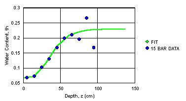
Notice that the 1500kPa (or 15.306 m or 15 bar) data in Table 2 were not developed either at the same depths in the soil column, or to the deepest depth in Table 1. The data were fitted (Figure 1) with a Gompertz function [1], and extended to 137 cm (Table 3). Unfortunately, it is apparent in later discussion that the 15-bar data do not always seem to be in the same data set as the pressure plate data.

[1]

Figure 1: Plot of 15 bar water content (cm3/cm3) data (points, Table 2) and fitted equation (line, Table 3) versus depth (cm)

Table 3: 15-bar Water contents, th (cm3/cm3), fitted to depth, z (cm), by [1]
z	th	z	th	z	th
0	0.0670	61	0.2083	122	0.2297
15	0.0719	76	0.2220	137	0.2299
30	0.1144	91	0.2271
45	0.1725	106	0.2290

It should also be noted that the water content data for z = 0 cm in Table 1 was not developed on a pressure plate apparatus. It was calculated from the bulk and particle densities, because of the difficulty of getting the samples fully saturated. This means that there is an unknown systematic error between this saturated water content, ths, and the remaining unsaturated water contents, th(z) in the table. The unsaturated water contents involve some unknown residual air content in the finest pores that did not exist for the saturated water content, ths. As the water is withdrawn from the soil in the pressure plate apparatus, these fine pores may or may not be eventually exposed to the contiguous air phase. There is no way to know where in the data this may happen. It also seems likely the that 10-bar and 15-bar measurements may have exposed these fine pores, where the lower suction measurements did not.

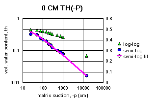
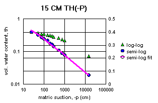
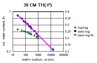
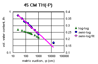
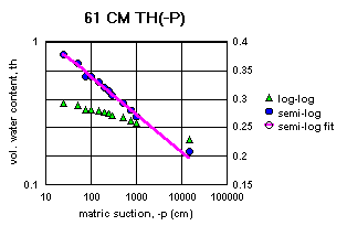
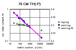
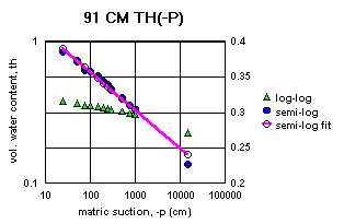
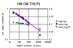
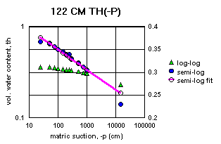
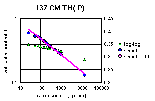
Figure 2a-j show the measured saturation relation data from Table 1 in log-log and semi-log plots, along with a line demonstrating a fitting equation [2], using the parameters in Table 4. Notice that for this equation, th can go to zero. The last column in Table 4 shows the matric suctions for this case. One could also choose to use the Brooks-Corey relation [3] or the van Genuchten-style relation [4]. But the approach for modeling the hydraulic properties of the soil column in this experiment and calibrating the model requires that the saturation relation be of the same form down the entire column. Only one of these can be chosen.

Figure 2a	Figure 2b
Figure 2c	Figure 2d
Figure 2e	Figure 2f
Figure 2g	Figure 2h
Figure 2i	Figure 2j

Figure 3: Soil water content, fitted by [2] with the Table 4 parameters, versus the measured water content for all the points in Table 1, plus the 15-bar points in Table 3.

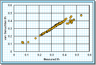
Since some of the log-log plots of measured data in Figures 2a-j can be well fitted with a straight line, the Brooks-Corey could be the best in those cases. But others have an obvious curvature in the log-log plots that would seem to demand a van Genuchten-style relation. Table 5 shows the fitted parameters for the standard van Genuchten relation [5]. Figure 4 shows the comparison of the fitted values to the measured values. Notice that the standard van Genuchten fit does very well except for saturated porosity, ths. In many cases it produces a lower value. There are duplicate values in Table 5 to demonstrate the pseudo-random nature of the simulated annealing method to make the fits (explained later).

Table 5: Fitting parameters for the van Genuchten saturation relation [5] and the measured data in Table 1. Fitted by simulated annealing with duplicate fits for some depths. Last column is the mean absolute error (MAE) of the fit to the measured data.
depth set z (cm)	ths (cm3/cm3)	thr (cm3/cm3)	at (cm)	m	n	MAE (cm3/cm3)
0	0.4707	0.0000	122.83	0.21847	1.27954	0.0094
0	0.4711	0.0000	119.72	0.21623	1.27589	0.0094
15	0.4168	0.0000	77.57	0.19237	1.23819	0.0054
15	0.4107	0.0000	97.01	0.20320	1.25502	0.0054
30	0.3745	0.0000	89.29	0.17928	1.21845	0.0032
30	0.3745	0.0000	89.09	0.17919	1.21831	0.0032
45	0.4029	0.0731	33.56	0.16321	1.19504	0.0025
45	0.3891	0.0887	48.15	0.18067	1.22050	0.0025
61	0.4093	0.0261	20.83	0.10146	1.11291	0.0017
61	0.4041	0.0651	27.62	0.12032	1.13678	0.0018
76	0.3867	0.0000	45.40	0.08704	1.09534	0.0017
91	0.3864	0.0000	96.80	0.09503	1.10501	0.0021
91	0.3861	0.0000	99.32	0.09534	1.10539	0.0021
106	0.3670	0.0000	242.73	0.10202	1.11360	0.0019
106	0.3670	0.0001	243.08	0.10207	1.11367	0.0019
122	0.3662	0.0000	203.70	0.09707	1.10750	0.0015
122	0.3662	0.0019	204.30	0.09769	1.10826	0.0015
137	0.3982	0.0000	102.94	0.09884	1.10968	0.0012
137	0.3982	0.0005	103.25	0.09903	1.10991	0.0012

Figure 4: Van Genuchten fits [5] generated for data in Table 1 by the parameters in Table 5, versus the measured data in Table 1.

All of the semi-log plots in Figures 2a-j demonstrate that the simpler log relation [2] can fit the data in Table 1 as well as the van Genuchten relation [5], with all of the same values of ths. It has the added advantage that it does not require a parameter for the residual saturation, thr, making it the least number of parameters to fit. It is also reasonable to assume that if the saturation in [2] goes to zero, then so does the hydraulic conductivity, sc (cm/hr). This can produce some difficulties in the simulation model with stability and convergence. If the displacement pressure parameter, at, is not changed in the model calibration, then Table 4 shows that equation [2] fits the entire range of the measured tensiometer readings for this experiment, at each depth (not shown here). Thus, any adverse effects from using equation [2] may not appear, or if they do, not in all the ranges of the possible parameter values (the parameter space).

Calibrating a model to a field experiment (Scott, et al., 1995) over a nominal growing season of more than 200 days is computationally intensive. Consider simulated annealing (Goffe, et al., 1994), with eight fitting parameters in a model that takes about 2 minutes to simulate 1-D infiltration and evapotransipration in a 225-day growing season. It takes about 131 steps to go from an annealing temperature of 10 to 10^-5, with a reduction factor of 0.9. Suppose that the model is run 20 times with random parameter settings, before the step size is change, and that 10 such sets are run before the temperature is reduced. This means that it will take 132*8*10*20*(2(min))/(60*24) = 293.3 days of computer time to reach a resolution, 68 days longer than the growing season being simulated.

This makes choosing a saturation relation with the least number of fitted parameters, along with some other optimization method, a reasonable first approach. In addition, the curvature in the log-log plots of measured saturation data is slight, and there are not enough data points in the low and high matric suction ranges. That makes it difficult to clearly and independently identify the at, vm and vn parameters in the van Genuchten-style relation [4], which in the fits tried, behaved as an equation with too many variables.

Fitting Saturation Relations with Simulated Annealing  (top)

While the computational overhead of simulated annealing (Goffe, et al., 1994) is burdensome for model calibration, it works quite well for fitting saturation relations. For those wishing a better understanding of the process, additional readings may include Corana, et al. (1987), and Kirkpatrick, et al. (1983). A public-domain Fortran program, simann (http://netlib.bell-labs.com/netlib/opt/simann.f.gz), associated with Goffe, et al., was modified to perform the fits presented in Tables 4 and 5.

Simulated annealing is a numerical optimization process that imitates the cooling of metal from high to low temperature. As metal cools, its atoms vibrate less and less, eventually "freezing" into their final positions. If the metal is quickly quenched, its atoms may be caught in positions that are not optimal in terms of the lowest possible energy. It may thus contain stresses and coarse grain structures, literally frozen into position. But if the metal is cooled very slowly, its atoms may naturally find the positions of lowest energy and stress.

Numerical simulated annealing is a pseudo-random process. Say that the "energy" of a data system is represented by a measure called an objective function. In this case, it is the sum of the absolute errors of the fitted saturation relation relative to the measured volumetric water content. The fitting parameters are always given a starting point, a first estimate. In this case, the program allows the user to make the first estimate, or will make the estimation itself.

The program is allowed a certain range of movement in the parameter space, a step length, within fixed limits. From the first point, it will take the each parameter and make a step away from it a random distance that is less than one-half the step length. If the objective function is lower, this will be the new best point and new starting point for the next step. If the objective function is higher, it may or may not accept the new point as the starting point for the next step, depending on the annealing temperature, which starts high.

The annealing temperature is used in an second pseudo-random process that accepts larger increases in the objective function for larger annealing temperatures, with an exponential probability. The higher the annealing temperature, the more likely a parameter point with a "worse" objective function value will be accepted as the start of the next step. Between random step lengths, and the random acceptance of worse values, the process has a good but finite chance of stepping out of local minima of the objective function to find the universal best minimum, the global minimum.

There are other details of the method that are left to the references. The step length is adjusted after 10 steps of each parameter to eventually become very small, and thus specify the resolution of the method. After each 200 steps of each parameter, the annealing temperature is reduced, decreasing the probability that a worse point will be accepted. The overall best point in each temperature cycle is retained as the starting point for the next cycle. Eventually, when both the temperature and the step sizes are very small (10^-6), the best overall point is taken as the final result.

As the data in Table 5 demonstrate, the pseudo-random nature of the process does not guarantee the same answer every time. This is almost guaranteed in the program discussed here, satfitsa.exe, by using the computer clock time to seed the random number generator. Thus, the answers will most likely not be exactly the same in every run, even with the same input data and first estimates. The advantage of this is that a slightly better estimate might be found with more runs.

The computer program, satfitsa, will fit three types of saturation relations, the five-parameter van Genuchten-style relation [4], the three-parameter log relation [2] and the four-parameter standard van Genuchten relation [5]. It will allow the user to select the initial starting estimates for the parameters, or make its own estimates from the data. If the program is allowed to make its own estimates, it is wise to have a full range of data, and ten points or more. Please note that the program runs only under MS- or other compatible DOS, or in a DOS window in Windows. The input and output files are DOS ascii files.

The program will begin by asking for three filenames, one input and two output files. They must all be in DOS 8+3 filename format, with 8 or less characters, optionally followed by a dot and three or less characters. Table 6 shows the format of the input file. Except for the "series" identifier, all of the data is unformated, and must be set up on each line as shown. The x1 to x5 variables are the input estimates for the fitting parameters, designated under usage, and must all contain values, even if they are unused dummy variables.

Table 7 shows the output format for the long output file, of the second name requested by the program at start. It adds to the basic input data. The names of the input and output files are added at the beginning to help in spreadsheets. The values the water content calculated by the fitting equation, th-fit, are added to the input (y, th) points on the same line, to use in spreadsheet plots. The input estimates of the parameter values are replaced by the program optimal values, followed by the final step sizes, res1 to res5, used in searching for the optimum. The magnitudes of these step sizes are a reliable indicator of the resolution of the optimal parameter values. Finally, the objective function, f, the summed-absolute-error of the fitted points, shows the overall error of the fit.

The short output file, of the third filename requested by the program at start, tabulates the results without the data points. It contains one line for each input data set. If the fitting method is 1 or 10 (equation [4]), the line is:

If the method is 2 or 20 (equation [2]), the line is:

series, ny, ier, me, th(1), th(2), ths, 0, at, vn, 0, fopt, res(ths), res(at), res(vn), 0, 0

If the method is 3 or 30 (equation [5]), the line is:

series, ny, ier, me, th(1), th(2), ths, thr, at, m, n, fopt, res(ths), res(thr), res(at), res(n), 0

The variables th(1) and th(2) are the first and second water contents of the input (y, th) points, for comparison to the ths value.

Table 8 shows the upper and lower limits allowed for the parameters by the program. Any user estimates outside these limits will be adjusted inside. Please note that the matric suction, y, is in the dimensions of meters. Please make any changes in scale necessary before and after the program runs.

Table 8: Upper and lower limits for fitted parameters
Method 1 or 10	Method 2 or 20	Method 3 or 30
, y(1) = 0 is taken to be a saturation measurement
0 £ thr £ 0.999 th(ny)	---	0 £ thr £ 0.999 th(ny)
10-4 £ at £ 5	10-4 £ at £ 5	10-4 £ at £ 10
1 £ vm £ 15	10-3 £ vn £ 10	---
0.1 £ vn £ 15	---	0.1 £ n £ 20

Associated files available for downloading:  (top)

1. satfitsa.exe - MS-DOS executable program to fit three saturation relations (73k).
2. se030001.dat - example DOS ascii input file for satfitsa; contains the data from Table 1 twice, set up for program estimates and fitting to the standard van Genuchten function [5] (the parameter estimates in the file are not used, and a good thing, too) (7k).
3. se030002.prn - example long output file generated by satfitsa from se030001.dat (14k).
4. se030003.prn - example short output file (4k).
5. se030002.123 - example Lotus 1-2-3 97 spreadsheet file with a graph (Figure 4) demonstrating the data (30k).
6. se010001.123 - example Lotus 1-2-3 spreadsheet file with the data and graphs used to generate Figures 2 and 3 (98k).
7. satfitsa.zip - a zipped file with all of the files above (60k).

Conductivity Relation Fits  (top)

It is not entirely clear from Theisse's thesis (1984) and notes how he used the experimental data from the plane of zero flux method (Arya, et al., 1975) to generate his unsaturated conductivity relationships. He gives the unsaturated conductivity relation [6] and the tabular values of A and B (Table 9) from an unspecified averaging method over 12 plots at the given depths. Equation [6] can also be expressed as [7], where the saturated conductivity, sc (cm/h), and the saturated water content, ths (cm³/cm³), are explicitly parameters. If one substitutes the log saturation relation [2] into [7], one obtains [8], which makes the unsaturated conductivity, ck, an explicit function of the hydraulic pressure, p (cm). It produces two fitting parameters, sc and bc (dimensionless) that are independent of the saturation relation.

Notice that in order to develop equation [7] for each of the soil depths, one must have values of ths, A and B at the same depths. Unfortunately, the depths in Table 9 do not match the depths in Table 1 or Table 4. But the two sets of depths are positioned midway between each other, making simple averaging a reasonable approximation. For values outside the available ranges, such as z = 0 for A and B, and z > 114 for A and B, and z > 137 for ths and vn, let us simply extend the nearest value that is available, and produce a set from z = 0 to z = 201 cm.

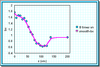
Figure 5a shows the parameters B and vn cross-interpolated to the same z-points. Figure 5b shows the points generated from B× vn, and a smoothed line of bc through the points. The smoothed line was generated by TableCurve 2-D (SPSS, Inc), using a 21.1% Loess smoothing spline method. Table 10 shows the points taken from the curve to use in the model.

Figure 5a: Cross-interpolated B and vn	Figure 5b: bc = B*vn, and and spline-smoothed

References  (top)